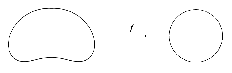
Example of biholomorphism, as described by the Riemann mapping theorem.
The Riemann mapping theorem is one of the most central results in complex analysis. However, the standard proof [1] lacks intuition. We will see an intuitive proof using ideas from topology and partial differential equations (PDEs). No background in topology or PDEs is assumed. However, I will state and use (without proof) some theorems from topology that are intuitively obvious, even though their proofs are nontrivial. I will refer to these theorems as i.o., and in the final section I will provide references for their proofs.
To the hesitant student of mathematics: it is a standard practice among mathematicians to use established i.o. theorems, without having seen the proof. This is because they want to use their time to focus on the more conceptual and creative aspects of their work.
Prerequisites. The reader is expected to be familiar with undergraduate complex analysis up to the Cauchy integral formula (e.g., Chapters 1 and 2.1–2.4 from [1]).
We begin by introducing some definitions.
Paths and loops. Let \(a>0\). A continuous function \( p:[0,a] \to \mathbb{C} \) is called a continuous path. If \(p\) is also injective, we call it simple. A continuous path \( p:[0,a] \to \mathbb{C} \) is called a loop if \( p(0) = p(a). \) A simple loop is also called a Jordan curve. Finally, regarding paths that go to infinity, we will only need the following type: we say that \(p:(0,a) \to \mathbb{C}\) is a simple continuous path that starts and ends at infinity if \(p\) is continuous and injective, and \( p(t) \to \infty \) as \( t \to 0 \) or \( t \to a \).
We will need the following i.o. theorem about Jordan curves. If you are unaware of the term connected component, you can see [6].
Before stating the main theorem, we introduce one more concept.
Biholomorphisms. Let \(A, B\subseteq \mathbb{C}\) be open. If a holomorphism \(f:A\rightarrow B\) is a bijection, then we say that \(f\) is a biholomorphism. We will prove momentarily that if \(f\) is a biholomorphism, then its inverse is holomorphic. If there exists a biholomorphism between two open sets \(A, B\), then we say that \(A\) and \(B\) are biholomorphic.
Example of biholomorphism, as described by the Riemann mapping theorem.
We will prove a slightly simplified version of Theorem 2. This is in order to focus on the main ideas, without being distracted by the technical details needed for the fully general case. In [2], the authors generalize the approach we take here, to prove Theorem 2 in its full generality.
We prove Theorem 2 under the following assumption:
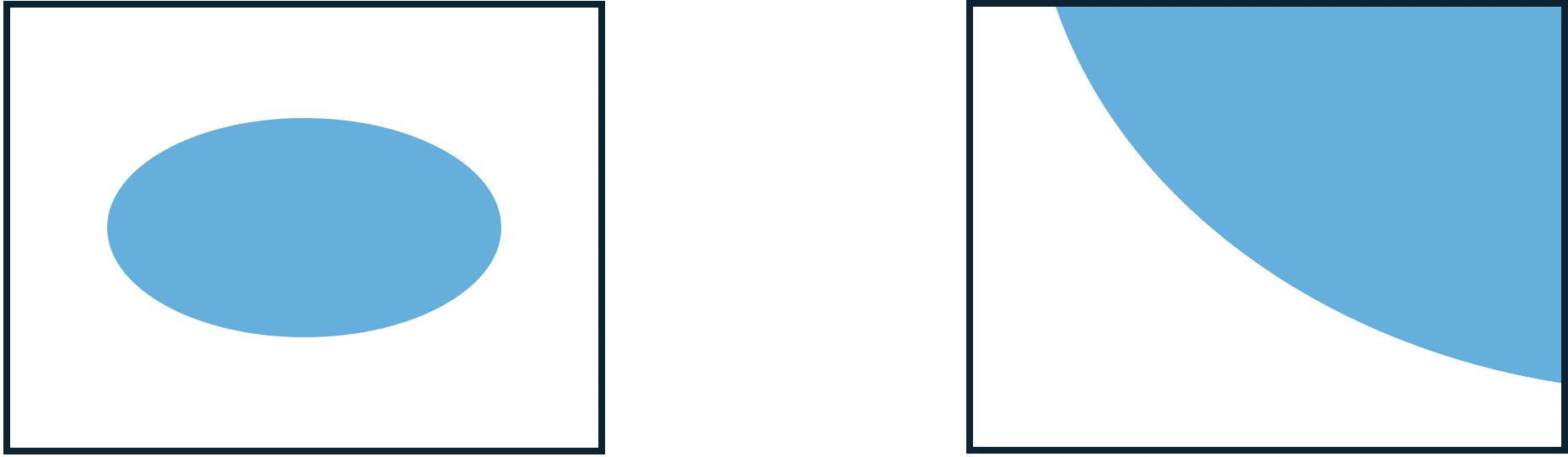
A bounded and an unbounded set satisfying our assumption.
Note that not all sets \(A\) in Theorem 2 satisfy our assumption, e.g., \(\mathbb{C}\setminus \{z\in \mathbb{C}: Re(z)\ge 0\}\).
We will first do the proof for the bounded case. Then, we will prove the unbounded case by a simple reduction to the bounded one.
We will need some tools to attack the bounded case. The first tool is topological and complex-analytic. It is called the argument principle, and it is covered in this article of mine. Even if you are familiar with it, you will most probably benefit from that article, since the proof is fully visual. We will also need two applications of the argument principle, covered here. Make sure you have understood the material from these articles, before you continue.
The third tool is the following theorem:
In PDE terms, this theorem says that the Dirichlet problem for the Laplace equation, on a domain bounded by a Jordan curve, has a unique solution. Theorem 3 has a very intuitive proof using probability theory. Even though the full proof requires an advanced concept called Brownian motion, the core idea can be described in elementary terms — and the solution \( u \) can actually be constructed in a fully elementary way! I suggest you accept Theorem 3 as a fact for now and continue with the rest of the article. When you're done, if you're interested in understanding how Theorem 3 is proved, then:
Now, let's move on with the proof of the bounded case.
Without loss of generality, we assume that \(0\in A\) (otherwise we can just translate \(A\)). We will construct a biholomorphism that sends zero to zero. First, we need a definition. Let \(\bar{S}\) denote the closure of a set \(S\).
The first thing we will do is deduce some properties satisfied by all strong biholomorphisms \(f:\bar{A}\rightarrow \bar{D}\) with \(f(0)=0\). These properties will give us insight into how to actually construct a biholomorphism from \(A\) onto \(D\) satisfying \(f(0)=0\). This function will in fact be a strong biholomorphism, but we will not prove this here, as it is not needed for our theorem.
Again, it is possible to show that \(\text{Im}(H)\) can also be continuously extended to \(\bar{A}\), which implies that the identity \(f(z)=ze^{H(z)}\) holds on \(\bar{A}\). However, we won't need this fact and so we won't prove it here.
Let \( g : \bar{A} \to \mathbb{C} \) be defined as
I claim that \( g \) is holomorphic on \( A \) and continuous on \( \bar{A} \). Indeed, locally around zero,
Thus, locally around zero,
So, \( g \) is holomorphic at zero, and clearly it is also holomorphic everywhere else on \( A \). The continuity of \( g \) at points of \( \partial A \) follows from the continuity of \( f \).
Now, from Theorem 2 in this article, we know that \( f' \neq 0 \) on \( A \). Furthermore, since \( f \) is injective, we have \( g \neq 0 \) on \( \bar{A} \). This implies that there exists a holomorphic function \( H : A \to \mathbb{C} \) such that \( g(z) = e^{H(z)}, \) for all \( z \in A \). For a proof of this implication, you can see [4].
Let \( u(z) \) and \( v(z) \) be the real and imaginary parts of \( H \). Since \( g \) is continuous on \( \bar{A} \) and \( u(z) = \ln(|g(z)|) \), the function \( u(z) \) can be continuously extended on \( \bar{A} \). \(\ \square\)
Continuing on the setting of Claim 1, we have that on the set \(A\), \(f(z)=ze^{u(z)+iv(z)}\), and so
for all \(z\in A\). Since \(f\) and \(u\) are continuous on \(\bar{A}\), the above equality extends on \(\partial A\). Now, the crucial moment: since \(f\) is a strong biholomorphism, we have \(f(\partial A)=\partial D\). This property actually tells us how to construct the function \(u\). Indeed, since \(|f(z)|=1\) on \(\partial A\), we have that \(u(z)=-\log |z| \), for all \(z\in \partial A\). But \(u\) is the real part of a holomorphic function on \(A\), and thus it is harmonic on \(A\). This means that we can construct \(u\) by solving this Dirichlet problem!
What about \(v\)? We can construct it by using \(u\)! Remember that these are coupled by the Cauchy-Riemann equations: \(u_x=v_y\) and \(u_y=-v_x\). Geometrically, this means that \(\nabla v\) is \(\nabla u\) rotated by \(90^\circ\) counter-clockwise. Since we have \(\nabla v\), we can get \(v\) up to an additive constant:
Thus, as long as there exists a strong biholomorphism \(f:\bar{A}\rightarrow \bar{D}\) with \(f(0)=0\), this function \(f\) is uniquely determined up to a rotation (expressed by the constant \(v(0)\)).
We now use these insights to construct a biholomorphism from \( A \) onto \( D \). Let \( u \) be the unique function that is harmonic on \( A \), continuous on \( \bar{A} \), and equals \( -\log |z| \) on \( \partial A \). Let
where \( \gamma \) is any piecewise-smooth curve that starts at the origin, ends at \( (x, y) \), and lies entirely inside \( A \). We will prove that the function \( f : A \to \mathbb{C} \) defined as
is holomorphic, sends \( A \) onto \(D \), and is injective. The fact that \( f \) is holomorphic is immediate, since \( u \) and \( v \) satisfy the Cauchy-Riemann equations (why?). We now prove the rest.
To highlight the main idea, we first do the proof under the assumption that \( f \) can be continuously extended on \( \bar{A} \). We then drop this assumption by tweaking our argument. As I mentioned in this article, whenever I say "argument principle", I mean its general version, given in Corollary 1 of that article.
Let \( \ell : [0,a] \to \mathbb{C} \) be a positively oriented Jordan curve that parametrizes \( \partial A \). By the way we constructed \( u \), we have \( f(\partial A) \subseteq \partial D \), and so the loop \( f \circ \ell \) lies entirely on the unit circle. This implies that \( |f(z)| \leq 1 \) for all \( z \in A \). Indeed, if \( |f(z_0)| > 1 \) for some \( z_0 \in A \), then by the argument principle \( W(f \circ \ell, f(z_0)) \geq 1 \), a contradiction. Since \( f \) is an open map , we have \( f(A) \subseteq D \).
We need to show that \( f \) is onto and injective. We will see that these are also consequences of the argument principle. What is \( W(f \circ \ell, 0) \)? By the argument principle, it equals the number of roots of \( f \) in \( A \), counting multiplicities. Clearly, zero is the only root of \( f \). Combining this with
we have \( W(f \circ \ell, 0) = 1 \). By Proposition 1 in this article, we have
for all \( q \in D \). By the argument principle, for each \( q \in D \), there exists exactly one \( z \in A \) such that \( f(z) = q \). \( \ \square\)
We now explain why for all small enough \(\delta>0\), the loop \(f\circ \ell_\delta\) is very close to the unit circle. Since \(u\) is continuous on the boundary, we can continuously extend \(|f|\) on \(\bar{A}\). Also, since \(\bar{A}\) is compact, \(|f|\) is uniformly continuous on \(\bar{A}\). This implies that for any \(\varepsilon>0\), there is a \(\delta_0>0\), such that for all \(\delta\in (0,\delta_0)\),
Using this fact, we can immediately adapt the proof we did under the continuity assumption. This adaptation is left as an exercise for the reader.
Let \( A \) be an unbounded, simply connected, and open subset of \( \mathbb{C} \) that is not the whole \( \mathbb{C} \). Suppose the boundary of \( A \) is a simple continuous path that starts and ends at infinity. We will construct a simple biholomorphism from \( A \) to a bounded, simply connected, and open subset of \( \mathbb{C} \), whose boundary is a Jordan curve. We proved that such a set is biholomorphic to \( D \). Thus, we will be able to conclude that \( A \) is biholomorphic to \( D \).
We will use the following i.o. theorem.
We apply this theorem to our setting. Without loss of generality, we assume that \(0\in B\) (otherwise, we can translate \(A\)). Let \(g(z):=1/z\). By applying \(g\) to the path \(p\), we get a Jordan curve. This is formally expressed by defining \( \tilde{p} : [0, a] \to \mathbb{C} \) as follows:
Observe that \(\tilde{p}\) is indeed a Jordan curve. By proving the following claim, we complete the proof of the unbounded case.
For completeness, I provide references for proving the i.o. theorems used in this article, and also in the one about the argument principle. As I said in the beginning, even though these theorems are intuitively obvious, their proofs are nontrivial. Several of them follow from a central theorem in topology called Jordan–Schoenflies (JS) theorem [7].
This article. Theorem 1 follows from JS (even though the first part is the simplest Jordan curve theorem). Theorem 4 follows from Theorem 1, by applying the inversion idea that we used for the unbounded case.
Argument principle article. Theorem 1 is proved using a topological concept called covering maps (see Chapter 9 of [8]). Theorem 4 also follows immediately from the techniques of that chapter, and it is the simplest example of a topological fact called Hopf’s Degree Theorem that is valid in any number of dimensions. Now, about Theorem 2, its first part is proven in Section 65 of [8], and the second part follows from the Annulus theorem [9], which is a consequence of JS. Finally, Theorem 5 follows from JS.