The Dirichlet problem for Laplace equation – or Dirichlet problem for short – is one of the most important partial differential equations. It goes as follows:
We will momentarily state a theorem that says that the Dirichlet problem has a unique solution, under a mild assumption on the set \( A \). There is a very intuitive way to prove this fact, using probability theory. Even though the full proof requires an advanced concept called Brownian motion, the core idea can be described in elementary terms, and the solution can also be constructed in a fully elementary way. This article is mainly for people who haven't studied Brownian motion, but want to understand the proof's main idea, along with the beautiful connection with probability theory. The probability prerequisites here are basic, and are covered in the first weeks of an elementary probability course.
The theorem will introduce a new term: that of a regular set. Immediately after, we discuss when a set is regular.
Even though we will not give here the full definition of a regular set, we will mention some sufficient conditions which imply regularity. These will showcase that pretty much all sets met in practice are regular. We start with a definition.
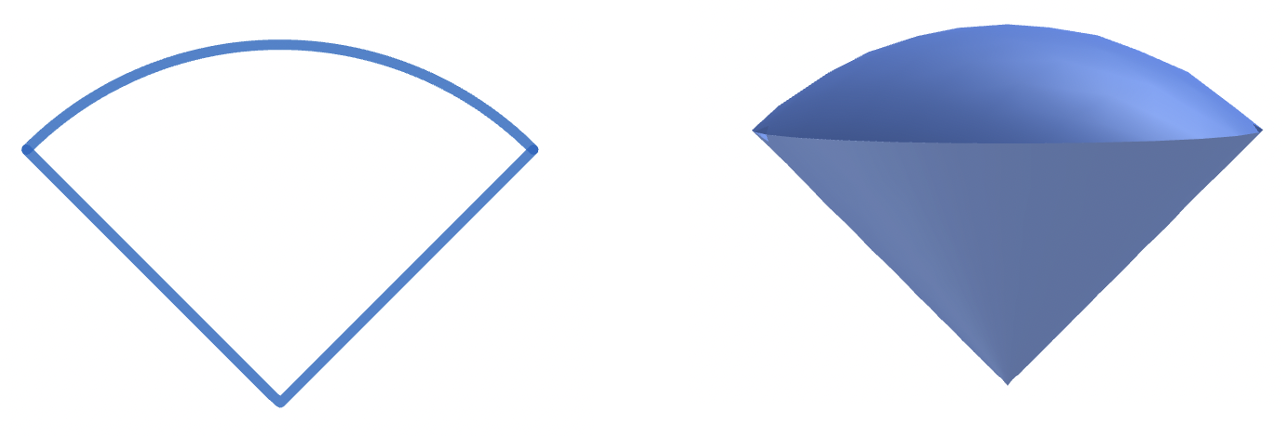
Definition of truncated cone. In \( \mathbb{R}^2 \), a truncated cone is simply a circular sector with angle between zero and 90 degrees. In \( \mathbb{R}^3 \), a truncated cone is the intersection of a cone with a ball centered on the cone's apex. The following figure shows examples of the two cases.
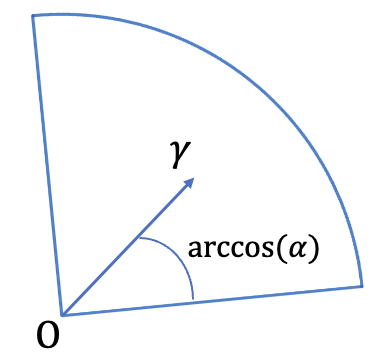
In \( \mathbb{R}^n \), we define a truncated cone with apex at the origin to be the set
\( \Gamma = \left\{ y \in \mathbb{R}^n : \alpha \|y\| < y \cdot \gamma,\ \|y\| < r \right\} \)
This set is parameterized by a unit vector \( \gamma \), and two numbers \( \alpha \in (0,1) \) and \( r > 0 \). The interpretation is that we take the intersection of the open ball centered at the origin with radius \( r \), and a certain cone. Which cone? The one that contains all vectors \( y \) whose angle with \( \gamma \) has cosine at least \( \alpha \). I.e., the angle is at most \( \arccos(\alpha) \).
A truncated cone with apex at a point \(x\) is a set \(x+\Gamma:=\left\{ x+y : y\in \Gamma \right\} \).
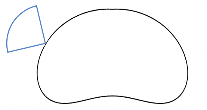
The cone condition. We say that an open set \(A\subseteq \mathbb{R}^n\) satisfies the cone condition if for every \(x\in \partial A\), there exists a truncated cone with apex at \(x\), that is disjoint from \(A\).
The first sufficient condition for regularity is this: if an open set \( A\subseteq \mathbb{R}^n \) satisfies the cone condition, then it is regular. Another condition (for two dimensions) is this:
Interiors of Jordan curves. If an open set \( A \subseteq \mathbb{R}^2\) is the interior of a Jordan curve, then it is regular. Observe that such a set does not need to satisfy the cone condition (consider for example the shape of a heart).
Proving Theorem 1 is done in two parts. The first is to show that a solution exists. The second is to show that we can't have two different solutions. The second is the easy part, and will be done in the last section of the article. We will now see the main idea for proving the first part. Specifically, the proof of existence is done in two steps.
The heart of the proof is step one. The second step, even though it requires considerable technical work, it is not that creative. Together, we will see the first step, and at the end I will say a few things about the second. We will first show how to construct the candidate solution for the case where \(A\) lies in \(\mathbb{R}^2\) and is the interior of a Jordan curve \(\ell:[0,a]\rightarrow \mathbb{R}^2\). After that, the generalization will be immediate. We start by interpreting the Laplacian of \(u\), i.e., the function \(\Delta u.\)
In the case of one variable, the Laplacian is just the second derivative. Let \( f : \mathbb{R} \to \mathbb{R} \) be twice differentiable. Then,
\[f''(x_0) = \lim_{\varepsilon \to 0} \frac{ \frac{f(x_0 + \varepsilon) + f(x_0 - \varepsilon)}{2} - f(x_0) }{ \varepsilon^2/2 } \]
This formula can be proven using Taylor's theorem. It gives an interpretation of the second derivative, i.e., the second derivative at \( x_0 \) measures how much \( f \) at \( x_0 \) differs from its average value at two symmetric neighboring points, close to \( x_0 \).
Applying this formula to the second partial derivatives, we can write the Laplacian as:
\[ \begin{align*} \Delta u(x_0, y_0) &= \frac{\partial^2 u}{\partial x^2}(x_0, y_0) + \frac{\partial^2 u}{\partial y^2}(x_0, y_0) \\ & \hspace{-1.8em} = \lim_{\varepsilon \to 0} \frac{1}{\varepsilon^2 / 4}\Bigg( \frac{u(x_0 + \varepsilon, y_0) + u(x_0 - \varepsilon, y_0)+u(x_0, y_0 + \varepsilon) + u(x_0, y_0 - \varepsilon)}{4} - u(x_0, y_0) \Bigg) \end{align*} \]
Thus, the Laplacian at \((x_0,y_0)\) measures how much \(u\) at \((x_0,y_0)\) differs from its average value at four symmetric neighboring points (right, left, up, and down), close to \((x_0,y_0)\). The formula also tells us that if \(u\) is \(C^2\), then the difference from the average will be \(O(\varepsilon^2)\). But, if \(u\) is harmonic, then it will be \(o(\varepsilon^2)\). So, intuitively a function is harmonic if at every point its value is very close to its average on such symmetric close neighboring points.
Remember, our quest is to construct a candidate solution. When we want to solve a tough problem, a useful strategy is to consider a similar one that is easier. By solving it, we will get new ideas about how to attack the original one. The simpler problem here will be the discrete Dirichlet problem.
Previously our space was \(\mathbb{R}^2\). Here it will be \(\mathbb{Z}^2\), i.e., the set of pairs of integers. Let \((i,j)\in \mathbb{Z}^2\). When we refer to the neighboring points of \((i,j)\), we mean the right, left, up, and down neighbors, i.e., the points \((i\pm 1, j)\) and \((i , j\pm 1)\). We begin with a definition.
Definition. A Jordan curve is called \(\mathbb{Z}^2\)-Jordan curve if it consists exclusively of line segments connecting neighboring points of \(\mathbb{Z}^2\).
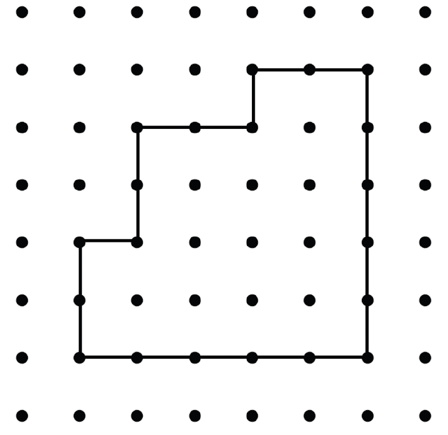
Example of a \(\mathbb{Z}^2\)-Jordan curve.
In the discrete Dirichlet problem, we are given a \(\mathbb{Z}^2\)-Jordan curve. Let \(L\) be the set of points of \(\mathbb{Z}^2\) that lie on that curve, and let \(A\) be the set of points of \(\mathbb{Z}^2\) that lie in its interior. We are also given a function \(g:L\rightarrow \mathbb{R}\). The goal is to find a \(u:A\cup L\rightarrow \mathbb{R}\) which is equal to \(g\) on \(L\), and also for all \((i,j)\in A\), \[ u_{i,j}=\frac{1}{4}\left(u_{i+1,j}+u_{i-1,j}+u_{i,j+1}+u_{i,j-1}\right) \tag{1} \]
The last condition is inspired by the interpretation of the Laplacian. In the continuous version it holds in the form of a limit, while here it is an equality. Observe that for each concept of the continuous Dirichlet problem, we have an analogous concept for the discrete, with the exception of the continuity of \(g\) and \(u\). We don't have an analogous concept for continuity here. The following theorem shows that there is no need for one:
We will only prove the existence here, since our goal is to show the analogous statement for the continuous problem. The uniqueness for the discrete problem will not be used anywhere in the article. To prove the existence, we will construct a solution using probability theory, and in particular random walks. If the reader has studied random walks, then they can skip the next subsection.

Consider the above segment, ranging from 1 to 10. Suppose we are at number 3, and we randomly jump to a neighbor, i.e., we go to 2 with probability 1/2 and to 4 with probability 1/2. Suppose we end up jumping to 4. Then, we jump again: to 3 or to 5, and we keep going like that. We stop when we reach the 1 or 10.
The question we want to answer is this: starting from 3, what is the probability of ending up at 1? We call this event \( S_1 \), and the goal is to compute \( P_3[S_1] \), where the subscript 3 indicates that we start at 3.
To compute this, we first generalize our notation: we denote by \( P_n[S_1] \) the probability of ending up at 1, if we start from the number \( n \). Thus, \( P_1[S_1] = 1 \) and \( P_{10}[S_1] = 0 \). For the other \( 1 < n < 10 \), we get from the law of total probability:
\[ P_n[S_1] = \frac{1}{2} P_n[S_1 \mid n \to n+1] + \frac{1}{2} P_n[S_1 \mid n \to n-1] \]
where \( n \to n+1 \) means that at the first move we go from \( n \) to \( n+1 \), and the same for the other transition. Observe that the probabilities on the right-hand side are simply \( P_{n-1}[S_1] \) and \( P_{n+1}[S_1] \). By denoting with \( a_n := P_{n}[S_1] \), we get:
\[ a_n = \frac{1}{2} a_{n-1} + \frac{1}{2} a_{n+1} \tag{2} \]
while \( a_1 = 1 \), \( a_{10} = 0 \). Thus, we have eight equations with eight unknowns. If you solve this system (you don't need to do this now; this is not the point), you will discover that the solution is unique, and in particular \( a_3 = \frac{7}{9} \).
The important thing in this example is not the result, but the form of equation (2)! It looks suspiciously similar to equation (1). We will use this connection to prove the existence part for the discrete Dirichlet problem.
Fix a point \( (i,j) \in A \). We define \( u_{i,j} \) as follows: we will do a random walk starting from \( (i,j) \), i.e., we will jump to one of its neighbors — right, left, up or down — with probability \( \frac{1}{4} \) each. After we jump, we do it again. We will stop when we reach a point on the boundary. Below we see an example of such a random walk.
Click to pause / resume.
Continuing with the definition of \(u_{i,j}\), let \(G_{i,j}\) denote the value of \(g\) at the boundary point reached by the walk (the subscript indicates the starting point and the capital \(G\) emphasizes that this is a random variable). We define
\[ u_{i,j} := \mathbb{E}[G_{i,j}] \tag{3} \]
Note that we could easily write a Python program to approximate this expectation, simply by running the random walk multiple times and averaging the values of \(g\) encountered at the boundary each time. Also, note that the definition of \(u_{i,j}\) in (3), even though we did it for \((i,j)\)'s in the interior, by extending it to the boundary, we immediately satisfy the condition of \(u\) being equal to \(g\) there. This is because a random walk starting on the boundary will immediately end. To establish that this \(u\) is a solution, we need to prove (1). Let \((i,j)\in A\). By the law of total expectation:
\[ \begin{align*} \mathbb{E}[G_{i,j}] &= \frac{1}{4} \mathbb{E}[G_{i,j} \mid (i,j) \to (i+1,j)] + \frac{1}{4} \mathbb{E}[G_{i,j} \mid (i,j) \to (i-1,j)] \\ & \ + \frac{1}{4} \mathbb{E}[G_{i,j} \mid (i,j) \to (i,j+1)] + \frac{1}{4} \mathbb{E}[G_{i,j} \mid (i,j) \to (i,j-1)] \end{align*} \]
where the conditioning is done on which neighbor we move to at the first step of the walk. But notice for example that the first conditional expectation on the right hand side is simply \(\mathbb{E}[G_{i+1,j}]\), and similarly for the other terms. This completes the proof of (1).
As we said, before constructing the solution for the general Dirichlet problem, we first do it in two dimensions, and with the set \(A\) being the boundary of a Jordan curve. Inspired by the solution for the discrete problem, we do the following construction. Let \(x_0\in A\), and let \(\varepsilon>0\) small. Starting from \(x_0\), we do a random walk of step \(\varepsilon\), where each step is right/left/up/down. When we do the step, we connect the current point with the previous with a linear segment, so that we have a continuous curve. We stop when this random curve hits the boundary for the first time, as in the animation below.
Click to pause / resume.
Let \(G_{x_0}^{(\varepsilon)}\) be the value of \(g\) at the point we hit the boundary. We define
\[ u(x_0) := \lim_{\varepsilon \to 0} \mathbb{E}[G_{x_0}^{(\varepsilon)}] \tag{4} \]
It can be proven that this \(u\) is indeed a solution. Before we say a couple of things about the proof, we will discuss an equivalent way to express it.
In probability theory, it is possible to define a random continuous curve, that starts from a point \(x_0\), and it is — in a certain sense — the limit of the above random walks as \(\varepsilon \to 0\). This random curve is called Brownian motion, and in the animation below, we see one realization of it.
Click to pause / resume.
If we let \(G_{x_0}\) to denote the value of \(g\) that the Brownian motion will meet the first time it hits the boundary, then it can be proven that \[ u(x_0) = \mathbb{E}[G_{x_0}] \tag{5} \]
Proving that (4) is indeed a solution. The modern way of doing this is by passing through Brownian motion. The high-level steps are 1) define Brownian motion, 2) prove some of its basic properties, 3) prove that (5) is a solution, and 4) prove that the expressions (4) and (5) are the same. Given this proof, the consideration of expression (4) seems unnecessary, since on the way of proving that it is a solution, we already establish the existence of one. However, the value of this expression is that a student with elementary probability knowledge can completely understand it.
General Dirichlet problem. Until now, we were working in two dimensions. Let \(A\subseteq \mathbb{R}^n\) be an open and bounded set, and let \(g:\partial A\rightarrow \mathbb{R}\) be a continuous function. The construction (4) immediately generalizes: instead of having four options at each step, we now have \(2n\). The Brownian motion–based construction also generalizes easily, as does the proof outlined above (assuming that \(A\) is regular). For the proof, the reader can consult [1].
Let \( A \subseteq \mathbb{R}^n \) be open and bounded (we won't need to assume regularity here). Let \( g : \partial A \to \mathbb{R} \) be continuous. We will show that we cannot have two different solutions to the Dirichlet problem. To do this, we first prove two basic properties of harmonic functions. Let \( \bar{B}_{x_0,r} \) denote the closed ball in \( \mathbb{R}^n \), centered at \( x_0 \), and of radius \( r \).
The proposition says that if a ball is inside \( A \), then the average of \( u \) on the ball (or on the sphere) equals its value at the center. Let's take a moment to appreciate this statement. Previously we saw that the average of \( u \) on the \( \varepsilon \)-neighbors of \( x_0 \) along the axes (4 neighbors in two dimensions, \( 2n \) neighbors in \( n \) dimensions) is very close to \( u(x_0) \). Here, we see that if the neighborhood is chosen to be a whole sphere or a ball (centered at \( x_0 \)), then we have exact equality. Furthermore, this neighborhood does not need to be close to \( x_0 \); the radius \( r \) is arbitrary!
Note that Proposition 2 does not exclude the possibility that the extreme values are attained in the interior. However, they must also be attained at the boundary.
The uniqueness follows immediately from the maximum principle: suppose we have two solutions \(u_1,u_2\). Then, \(u_1-u_2\) is zero on the boundary, it is continuous on \(A\cup \partial A\), and is harmonic on \(A\). Thus, \(u_1-u_2=0\).