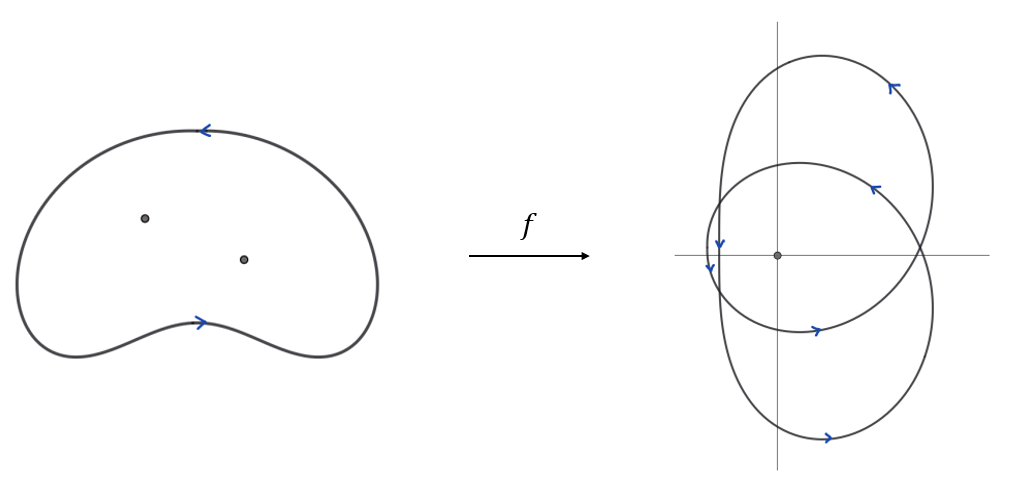
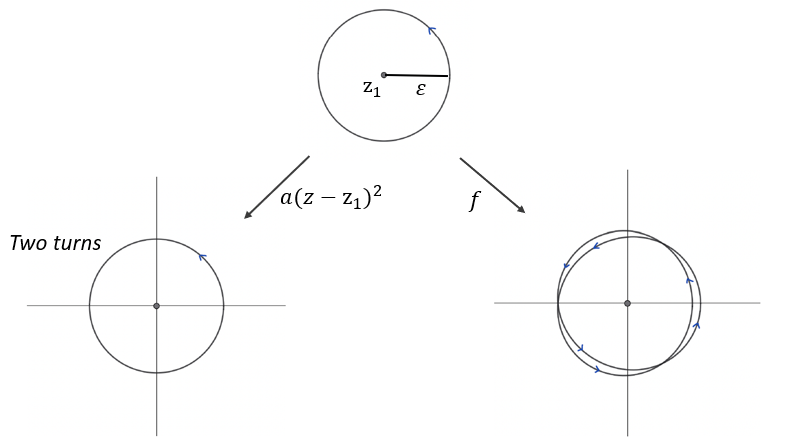
In this example we have two roots, on which \(f'\) is nonzero. We see that \(f(L)\) turns twice around the origin.
We start by recalling the definition of multiplicity of a root of a holomorphic function. Let \( A \subseteq \mathbb{R}^2 \) open, and let \( f: A \to \mathbb{C} \) be a holomorphic function. Let \( z_0 \in A \) be a root of \(f\), i.e., \( f(z_0) = 0 \). Suppose that not all derivatives \( f^{(k)}(z_0)\) are zero. We call the minimum \(k\) with \( f^{(k)}(z_0)\neq 0 \) the multiplicity of the root \( z_0 \). Note that if all these derivatives were zero and if \(A\) was connected, then \(f\) would be identically zero.
Before you go over this article, make sure you read the beginning of the Riemann mapping theorem article. Specifically, read up until Theorem 1.
The argument principle is a spectacular theorem that informally says the following (the formal version will follow momentarily): Let \( \ell:[0,a]\rightarrow \mathbb{C} \) be a Jordan curve. Let \(L:=\ell([0,a])\) be its image and \(A\) its interior. Let \( f \) be a continuous function on \(A\cup L \) that is holomorphic on \( A.\) Suppose also that \( f \) has no roots on \( L \). Then the number of roots of \( f \) in \( A \) (counted with multiplicities) is equal to the number of times \( f(L) \) turns around the origin.
In this example we have two roots, on which \(f'\) is nonzero. We see that \(f(L)\) turns twice around the origin.
We need to formalize the above statement. Given a loop \( \ell \) that does not hit zero (meaning \( \ell(t) \neq 0 \) for all \( t \)), the phrase “number of times \( \ell \) turns around the origin” is not a rigorous statement. Mathematics is built on set theory, not on our visual intuition (although it is inspired and guided by it). To make the phrase rigorous, we need an i.o theorem which establishes the existence of the angle function for a continuous path (for references containing proofs of the i.o. theorems used in this article, see the final section here).
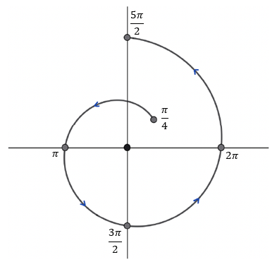
We call \( \theta_p \) the angle function of \( p \). Note that, as illustrated in the figure above, continuity may require \( \theta_p \) to take values outside of \([0, 2\pi)\). Let \( \Delta \theta_p := \theta_p(a) - \theta_p(0) \). This is the total angle swept out by \( p \). In the figure above \( \Delta \theta_p = 9\pi/4 \).
From Theorem 1, it follows that if \( \ell: [0,a] \to \mathbb{C} \) is a loop that does not hit zero, then \( \Delta \theta_\ell \) is an integer multiple of \( 2\pi \). For such a loop, we call the integer \[ W(\ell, 0) := \frac{\Delta \theta_\ell}{2\pi} \] the winding number of \( \ell \) around zero. This is the number of times \( \ell \) “turns around the origin.” Now, for a point \( z_0 \in \mathbb{C} \) and a loop \( \ell \) that does not hit \( z_0 \), we define \[ W(\ell, z_0) := W(\ell - z_0, 0) \] where \( \ell - z_0 \) is the loop \( \ell \) translated by \( -z_0 \).
There is one thing left to formalize the argument principle: we need to define what a positively oriented Jordan curve is. We begin with an observation:
Proposition 1. If \( p:[0,a] \to \mathbb{C} \) is a continuous path that does not hit zero, then the reverse path \( \bar{p}:[0,a] \to \mathbb{C} \), defined as \( \bar{p}(t) := p(a - t) \), satisfies \(\Delta \theta_{\bar{p}} = -\Delta \theta_p.\)
Exercise: use Theorem 1 to prove Proposition 1. Now, we will need the following i.o. theorem. This theorem uses the concept of continuous deformation of loops. If you are unaware of this term, click here.
Click to repeat. Example of deformation from Theorem 2.
Note that by taking the reverse of a Jordan curve we flip its orientation.
Now, observe that \(f\) has finitely many roots. Here is why: a standard result in introductory complex analysis is that since \(f\) is not identically zero, its roots have no limit point in \(A\) (for a proof, see [1]). Now, \(f\) is continuous and nonzero on \(L\), so the roots also have no limit point in \(L\). Since \(A \cup L\) is compact, the roots are finitely many. Let's call them \(z_1, z_2, \dots, z_n\) and their respective multiplicities \(m_1, m_2, \dots, m_n\).
We will break the proof into three steps. In each step, I first give an informal argument clarifying the underlying idea, and then I formalize it.
Suppose \(f\) has no roots in \(A\), and assume that \(W(f \circ \ell, 0)\neq 0\). Let \(\bar{A}:= A \cup L\). From Theorem 1 here, \(\bar{A}\) is simply connected and thus \(\ell \) can be continuously deformed to a point \(z_0 \in \bar{A} \) while staying inside \(\bar{A}\) (note that \(z_0\) can be trivially expressed as a loop \(\ell_0(t)=z_0\)). Consider the images of these deformations under \(f\). Since \(f\) is continuous, these images will comprise a continuous deformation of \(f \circ \ell\) to \(f(z_0)\). Since \(f\) has no roots, none of these loops hits the origin. This implies (by Theorem 4) that all of them turn around the origin \(W(f \circ \ell,0)\neq 0\) times. Since these loops shrink down to \(f(z_0)\), we must have \(f(z_0)=0\) (as in the animation below), contradiction.
Click to play/pause.
We will prove the argument principle for the restriction of \(f\) on a small disc of radius \(\varepsilon>0\) centered on some root; suppose it is \(z_1\).
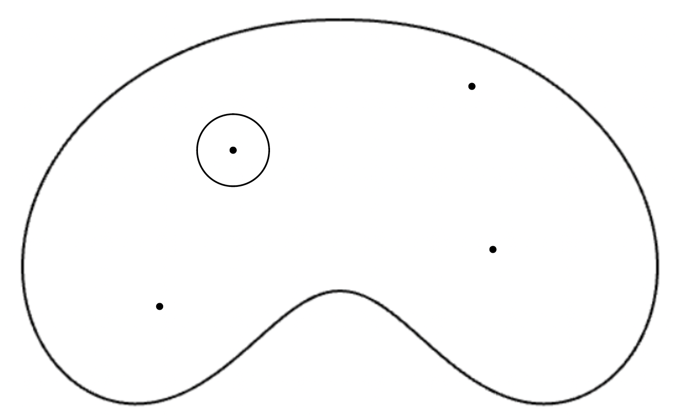
The corresponding circle is \(C_{z_1,\varepsilon}(t)= \varepsilon e^{i 2\pi t} + z_1\), \(t\in[0,1]\). We also denote by \(D_{z_1,\varepsilon}\) and \(\bar{D}_{z_1,\varepsilon}\) the corresponding open and closed discs. Now, from Taylor's theorem we have that for \(z\) close to \(z_1\), \[ f(z)=a(z-z_1)^{m_1}+E(z-z_1) \] where \(a= f^{(m_1)}(z_1)/m_1!\) and \(E\) is an error-function that is much smaller compared the leading term \(a(z-z_1)^{m_1}\). Specifically, \(E(z-z_1)\) is of the order of \(|z-z_1|^{m_1+1} \ll |a| |z-z_1|^{m_1}\), for \(z\) close to \(z_1\). Now, note that if we apply the function \(a(z-z_1)^{m_1}\) to the circle \(C_{z_1,\varepsilon}\), we get the circle centered at the origin and of radius \(|a|\varepsilon^{m_1}\), wrapped on itself \(m_1\) times. Since \(f\circ C_{z_1,\varepsilon}\) is a small perturbation of that loop (see figure below), we have \(W(f\circ C_{z_1,\varepsilon},0)=m_1\).
First, suppose \(f\) has only one root: \(z_1\in A\). Consider a small disc \(\bar{D}_{z_1,\varepsilon}\) contained in \(A\). We proved that \(W(f\circ C_{z_1,\varepsilon},0)=m_1\). From Theorem 2, we can continuously deform \(C_{z_1,\varepsilon}\) to \(\ell\) while staying in \(\bar{A}\setminus D_{z_1,\varepsilon}\). The images of these deformations do not touch the origin, and thus they all have the same winding number, as in the animation below.
Click to play/pause.
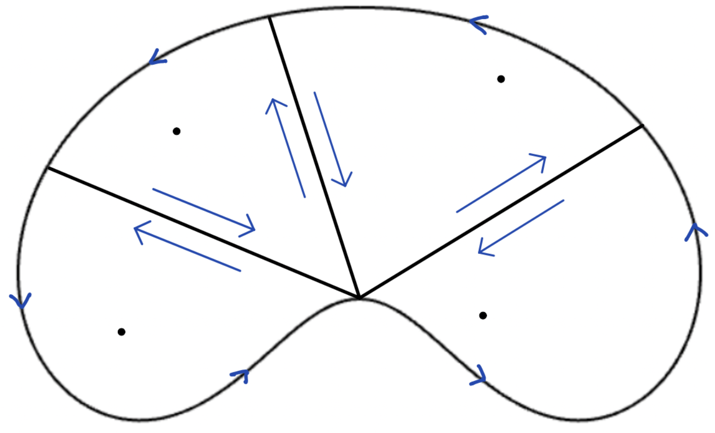
Suppose \(f\) has exactly two distinct roots \(z_1,z_2\). The idea here is to split \(\bar{A}\) into two pieces - each containing exactly one root - as in the figure below:
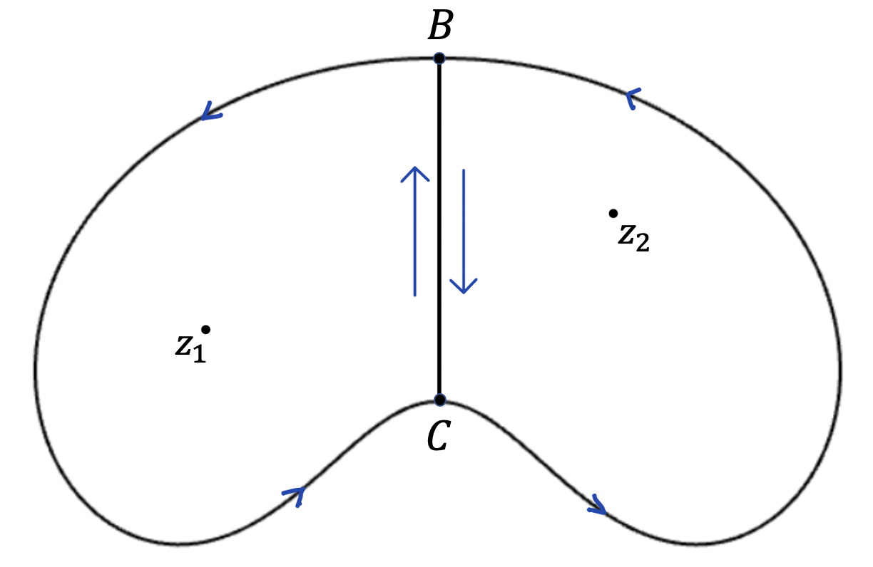
Let \(\ell_1:[0,1]\rightarrow \mathbb{C}\) be the positively oriented Jordan curve bounding the left piece and \(\ell_2:[0,1]\rightarrow \mathbb{C}\) the corresponding for the right piece. Let \(B\) be the point where both curves start and finish, i.e., \(\ell_1(0)=\ell_1(1)=\ell_2(0)=\ell_2(1)=B\). As we see in the figure, both \(\ell_1\) and \(\ell_2\) share the segment \(BC\), but they traverse it in opposite directions. From the case of one root, we know that \(W(f\circ \ell_1,0)=m_1\) and \(W(f\circ \ell_2,0)=m_2\). I claim that \(\Delta \theta_{f\circ \ell}= \Delta \theta_{f\circ \ell_1}+ \Delta \theta_{f\circ \ell_2} \). To see why, consider the loop \(\ell_1 * \ell_2\) that does this: starts from \(B\), goes around \(\ell_1\) and returns to \(B\), and then goes around \(\ell_2\). Let's study \(\Delta \theta_{f\circ (\ell_1 * \ell_2)}\). Since \(f\circ (\ell_1 * \ell_2)\) first traverses \(f\circ \ell_1\) and then \(f\circ \ell_2,\) we have \(\Delta \theta_{f\circ (\ell_1 * \ell_2)}= \Delta \theta_{f\circ \ell_1} + \Delta \theta_{f\circ \ell_2}\). On the other hand, the back-and-forth of \(f\circ (\ell_1 * \ell_2)\) on \(f(BC)\) contributes nothing on the total angle swept, and thus \(\Delta \theta_{f\circ (\ell_1 * \ell_2)}=\Delta \theta_{f\circ \ell}\). Having shown that \(\Delta \theta_{f\circ \ell}= \Delta \theta_{f\circ \ell_1}+ \Delta \theta_{f\circ \ell_2} \), we get that \(W(f\circ \ell,0)=m_1+m_2\).
If we have \(n\) distinct roots, we simply extend the above cancellation idea as in the figure below: